Box
License
Copyright (C) 2017 Dominic Walden. Permission is granted to copy, distribute and/or modify this document under the terms of the GNU Free Documentation License, Version 1.3 or any later version published by the Free Software Foundation; with no Invariant Sections, no Front-Cover Texts, and no Back-Cover Texts. A copy of the license can be found here: https://gnu.org/licenses/fdl.html.
The problem
- You are imprisoned in a pitch black, mostly featureless phonebox with a solid roof and floor
- There are four walls, with a waist-height hole in each with a button at the back; walls, holes and buttons are identical
- Each button starts randomly in one of two states and can be toggled by pressing the button; you do not know nor are you able to determine a button's state
- As an "action" you may insert your arm(s) into any of the holes and (simultaneously) press the button(s), then remove your arm(s)
- If all the buttons are now all in the same state, you escape
- If not, the phonebox spins around, eventually stopping but leaving you disorientated and with no indication as to which button(s) you just pressed
- There are no trick solutions accepted for the puzzle e.g. you can't mark walls, use your feet, etc.
- Can you guarantee your escape?
Solution
You can imagine the box like so:
        N
        ^
   +---------+
   +         +
   +         +
W  +         +  E
   +         +
   +         +
   +---------+

        S
Buttons are at N, E, S and W. Each one can be at position 0 or 1.
Starting with the button the front of the box is pointing at (indicated by the arrow), we can express the state of the buttons in four digits. For example,
1 0 0 1
would represent N=1, E=0, S=0, W=1.
There are 16 states in which the buttons can be at any time. Each one of these states can be represented in GNU Octave as a row vector:
[1, 0, 0, 1]
ans =

   1   0   0   1
As an action you can push one or two buttons, changing its state from 0 to 1 or
from 1 to 0. For example, from 0 1 1 0 pushing S and W buttons will get you
0 1 0 1.
Therefore, a random push of one or two buttons is a function from one four digit binary number to another.
function finalState = pushRandom (state)
With one finger there are 4 ways to push 4 buttons.
combn(c("N", "E", "S", "W"), 1)
     [,1] [,2] [,3] [,4]
[1,] "N"  "E"  "S"  "W"
With two fingers, there are \({4 \choose 2} = 6\) different ways.
combn(c("N", "E", "S", "W"), 2)
     [,1] [,2] [,3] [,4] [,5] [,6]
[1,] "N"  "N"  "N"  "E"  "E"  "S"
[2,] "E"  "S"  "W"  "S"  "W"  "W"
For a total of 10 different actions.
Each of these ways can also be expressed as a four digit binary number, with a 1
in each position of button you are pushing. For example, 0 1 1 0 represents
pushing E and S buttons.
Only binary numbers with one or two "1"s are possible as you can only push one or two buttons. Therefore, not all the 16 four digit binary numbers are possible.
allPushes = [1, 0, 0, 0
             0, 1, 0, 0
             0, 0, 1, 0
             0, 0, 0, 1
             1, 1, 0, 0
             1, 0, 1, 0
             1, 0, 0, 1
             0, 1, 1, 0
             0, 1, 0, 1
             0, 0, 1, 1];
Push one or two buttons at random. This will be the push state.
push = allPushes(randi(10), :);
To simulate pushing the buttons, xor the input state with the push state. Xor will flip 1 to 0 and 0 to 1 in any position where the push state has a "1".
finalState = xor(state, push);

endfunction
When the box spins around, the position of the arrow in the above diagram moves to N, E, S or W. It may spin more than 360°, but will still end up on one of those 4 positions. The state of the buttons relative to one another does not change, just their position in the sequence.
[Diagram]
For example, starting from 0 1 0 1 if the box spun 450° = 360 + 90 the arrow
will now be pointing at E and the button state will be 1 0 1 0.
[Diagram]
We will choose a number from 0 to 3 to represent ending in each position. Then use the shift function to do a circle shift of the state.
function finalState = shiftRandom (state)
  finalState = shift(state, randi([0, 3]));
endfunction
As mentioned above, there are 16 different starting states represented by 4 digit binary numbers. We will go through each in turn.
allStartStates = [0, 0, 0, 0
                  1, 0, 0, 0
                  0, 1, 0, 0
                  1, 1, 0, 0
                  0, 0, 1, 0
                  1, 0, 1, 0
                  0, 1, 1, 0
                  1, 1, 1, 0
                  0, 0, 0, 1
                  1, 0, 0, 1
                  0, 1, 0, 1
                  1, 1, 0, 1
                  0, 0, 1, 1
                  1, 0, 1, 1
                  0, 1, 1, 1
                  1, 1, 1, 1];
for startState = 1:16
Let's do 1000 experiments from each starting state.
for i = 1:1000
At the start you have not escaped and you have not done anything yet. Set the current state to the start state.
currState = allStartStates(startState, :);
escaped = false;
steps = 0;
While you are still in the box, your action is to push one or two buttons at random.
while (escaped == false)
  steps = steps + 1;
  currState = pushRandom(currState);
To escape, the state of all the buttons after pushing needs to be the same. This
means either all are "1" (i.e. 1 1 1 1) or not any are "1" (i.e. 0 0 0 0).
if (all(currState) | !any(currState))
  escaped = true;
Otherwise, the box spins and you go back to the start of the while loop.
  else
    currState = shiftRandom(currState);
  endif
endwhile
Once you have escaped, write the starting state and number of steps it took to a csv file and go back to the start of one of the for loops.
    csvwrite("random_tries.csv", [startState, steps], "-append");
  endfor
endfor
tries <- read.csv("random_tries.csv", header=FALSE)
summary(tries$V2)
 Min. 1st Qu.  Median    Mean 3rd Qu.    Max.
1.000   3.000   5.000   7.285  10.000  74.000
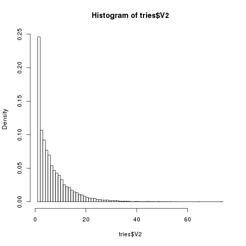
tries <- read.csv("random_tries.csv", header=FALSE)
hist(tries$V2, nclass=74, probability=TRUE)
tries <- read.csv("random_tries.csv", header=FALSE)
length(subset(tries, V2 == 1)$V2)
1
On the one hand I am very suspicious that the number of experiments ending in 1 steps is significantly lower than I predicted. On the other, the fact that most end in very few steps and that the histogram above looks so like a mathematical function seems to corroborate my hypothesis.
The function representing the probability of escaping in n steps would seem to be similar to f(n) = log(n).
After trying a few more runs of the experiment, I saw this odd output from R.
blah <- read.csv("random_tries1.csv", header=FALSE)
length(subset(blah, V2 == 1)$V1)
subset(blah, V2 == 1)
[1] 3
     V1 V2
1001  1  1
5001  5  1
9001  9  1
The fact that the times that it was happening in 1 step were always the first of the 1000 tries for the starting states made me realise that perhaps I was not setting the current state back to the starting state after the escape. This was in fact the case.
Indeed, this makes the above outcome predictable, as whenever the current state was one of the escape states (0 or 15) it is impossible to escape in one step.
graphics_toolkit ("gnuplot")
tries2 = dlmread("random_tries.csv", ",", 0, 1)
hist(tries2, 74, 1)
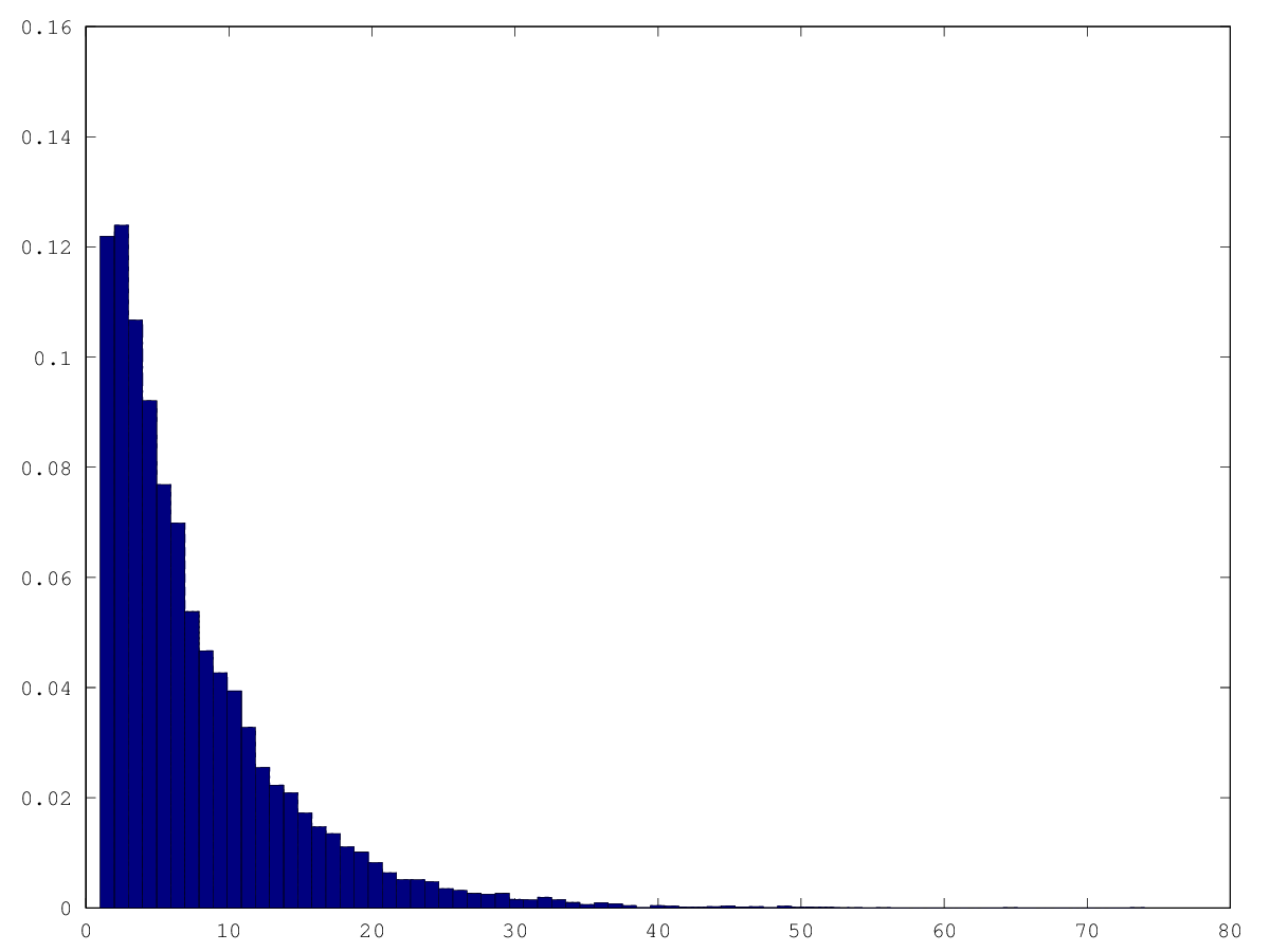
That looks better, although the figure for 1 seems incorrect. I do not think I am
using hist() correctly w.r.t. bin sizes.
Redoing the graphs in Octave gives me better results for bin size. The above graph appears to have got the correct y value for x=1.
With the exception of x=1 and x=2 the y values still appear to be decreasing logarithmically as I previously thought.
graphics_toolkit ("gnuplot")
tries2 = dlmread("random_tries.csv", ",", 0, 1)
stepsCounts = histc(tries2, 0:74)
cumStepsCounts = cumsum(stepsCounts)
cumProbSteps = cumStepsCounts / 16000
bar(0:74, cumProbSteps)
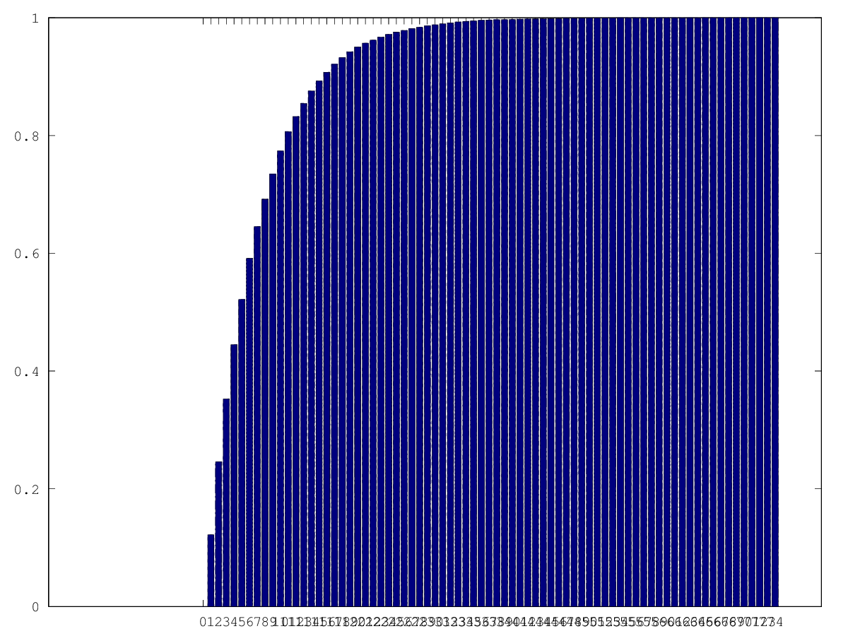
Each time there is a 1/7 average chance of pressing the right one or two buttons to escape. Therefore, the chances of getting to step n without escaping is 6/7^n.
function prob = pSteps (n)
  prob = 1 - (6/7)^n
endfunction
Comparing this with the data collected during the simulations and they appear to match pretty closely.
tries2 = dlmread("random_tries.csv", ",", 0, 1)
stepsCounts = histc(tries2, 0:74)
cumStepsCounts = cumsum(stepsCounts)
cumProbSteps = cumStepsCounts / 16000
What if you don't spin?
diff -w -u1 box.octave box_nospin.octave > diff.patch
cat diff.patch
--- box.octave	2016-12-31 17:02:53.241880505 +0000
+++ box_nospin.octave	2016-12-31 17:03:43.194128205 +0000
@@ -56,3 +56,3 @@
       else
-	currState = shiftRandom(currState);
+	## Stay where you are
       endif
@@ -60,3 +60,3 @@

-    csvwrite("random_tries.csv", [startState, steps], "-append");
+    csvwrite("random_tries_nospin.csv", [startState, steps], "-append");
   endfor
octave box_nospin.octave
tries <- read.csv("random_tries.csv", header=FALSE)
summary(tries$V2)
tries <- read.csv("random_tries_nospin.csv", header=FALSE)
summary(tries$V2)
 Min. 1st Qu.  Median    Mean 3rd Qu.    Max.
1.000   3.000   5.000   7.285  10.000  74.000
 Min. 1st Qu.  Median    Mean 3rd Qu.    Max.
1.000   2.000   5.000   7.169  10.000  77.000
Compared with the run with spinning, it does not appear to make a great deal of difference.
What if it is not random?
What if the spinning were not random?
What if the amount it spun you were a constant?
Each time, box is spun only 90 degrees.
diff -w -u1 box.octave box_spinconstant.octave > diff1.patch
cat diff1.patch
--- box.octave	2016-12-31 17:02:53.241880505 +0000
+++ box_spinconstant.octave	2016-12-31 17:52:29.800640463 +0000
@@ -21,3 +21,3 @@
 function finalState = shiftRandom (state)
-  finalState = shift(state, randi([0, 3]));
+  finalState = shift(state, 1);
 endfunction
@@ -60,3 +60,3 @@

-    csvwrite("random_tries.csv", [startState, steps], "-append");
+    csvwrite("random_tries_spinconstant.csv", [startState, steps], "-append");
   endfor
octave box_spinconstant.octave
tries <- read.csv("random_tries.csv", header=FALSE)
summary(tries$V2)
tries <- read.csv("random_tries_spinconstant.csv", header=FALSE)
summary(tries$V2)
 Min. 1st Qu.  Median    Mean 3rd Qu.    Max.
1.000   3.000   5.000   7.285  10.000  74.000
 Min. 1st Qu.  Median    Mean 3rd Qu.    Max.
1.000   3.000   5.000   7.231  10.000  57.000
No great difference apart from maximum number of steps.
What if there were some sort other pattern to the spinning?
Each step, the number of times the box spins increases by 90 degrees.
diff -w -u1 box.octave box_spinpattern.octave > diff2.patch
cat diff2.patch
--- box.octave	2016-12-31 17:02:53.241880505 +0000
+++ box_spinpattern.octave	2016-12-31 18:07:07.520992843 +0000
@@ -20,4 +20,4 @@

-function finalState = shiftRandom (state)
-  finalState = shift(state, randi([0, 3]));
+function finalState = shiftRandom (state, spins)
+  finalState = shift(state, spins);
 endfunction
@@ -56,3 +56,3 @@
       else
-	currState = shiftRandom(currState);
+	currState = shiftRandom(currState, steps);
       endif
@@ -60,3 +60,3 @@

-    csvwrite("random_tries.csv", [startState, steps], "-append");
+    csvwrite("random_tries_spinpattern.csv", [startState, steps], "-append");
   endfor
octave box_spinpattern.octave
tries <- read.csv("random_tries.csv", header=FALSE)
summary(tries$V2)
tries <- read.csv("random_tries_spinpattern.csv", header=FALSE)
summary(tries$V2)
 Min. 1st Qu.  Median    Mean 3rd Qu.    Max.
1.000   3.000   5.000   7.285  10.000  74.000
 Min. 1st Qu.  Median    Mean 3rd Qu.    Max.
1.000   3.000   5.000   7.224  10.000  60.000
As above, no significant difference apart from maximum steps.
I will look at their respective histograms.
graphics_toolkit("gnuplot")
tries = dlmread("random_tries_spinconstant.csv", ",", 0, 1)
hist(tries, 57, 1)

graphics_toolkit("gnuplot")
tries = dlmread("random_tries_spinpattern.csv", ",", 0, 1)
hist(tries, 60, 1)
None show anything of interest that I can see.
What if the button pressing were not random?
What if I approached it systematically? For example, trying each possible button press one after the other. I implement this by adding an extra argument to the "pushRandom" function which takes an integer stating which of the 10 possible button pushes to do. This integer has to be kept within the range of 1-10. There is a loop which will keep subtracting 10 from the number until it is less than 10.
diff -w -u1 box.octave box_pushsystematic.octave > diff3.patch
cat diff3.patch
--- box.octave	2016-12-31 17:02:53.241880505 +0000
+++ box_pushsystematic.octave	2017-01-01 11:21:19.085495615 +0000
@@ -1,3 +1,7 @@

-function finalState = pushRandom (state)
+function finalState = pushRandom (state, index)
+
+  while(index > 10)
+    index = index - 10;
+  endwhile

@@ -14,3 +18,3 @@

-  push = allPushes(randi(10), :);
+  push = allPushes(index, :);

@@ -50,3 +54,3 @@
       steps = steps + 1;
-      currState = pushRandom(currState);
+      currState = pushRandom(currState, steps);

@@ -60,3 +64,3 @@

-    csvwrite("random_tries.csv", [startState, steps], "-append");
+    csvwrite("random_tries_pushsystematic.csv", [startState, steps], "-append");
   endfor
octave box_pushsystematic.octave
tries <- read.csv("random_tries.csv", header=FALSE)
summary(tries$V2)
tries <- read.csv("random_tries_pushsystematic.csv", header=FALSE)
summary(tries$V2)
 Min. 1st Qu.  Median    Mean 3rd Qu.    Max.
1.000   3.000   5.000   7.285  10.000  74.000
 Min. 1st Qu.  Median    Mean 3rd Qu.    Max.
1.000   2.000   5.000   9.885  11.000 163.000
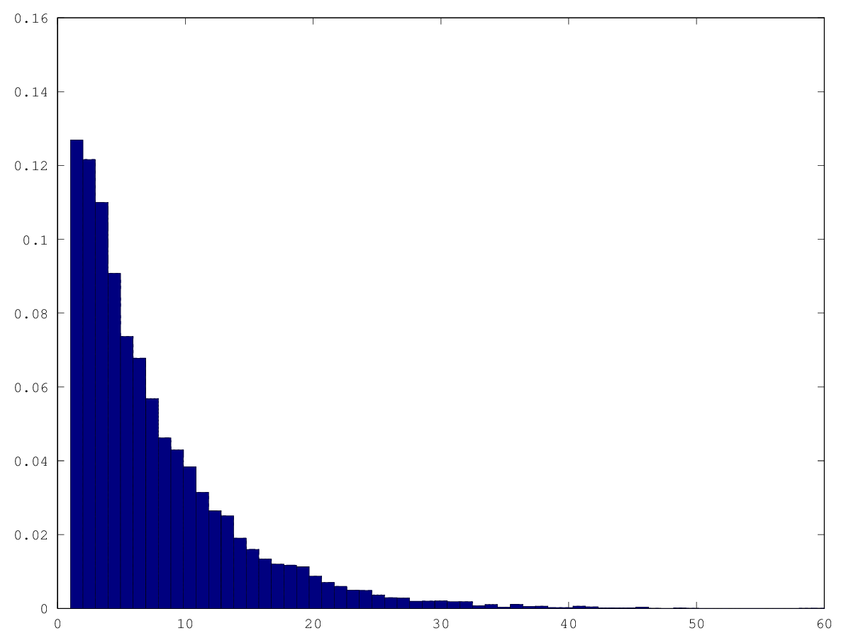
graphics_toolkit("gnuplot")
tries = dlmread("random_tries_pushsystematic.csv", ",", 0, 1)
hist(tries, 163, 1)
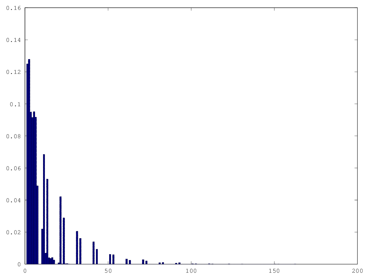
A more interesting shape. Similar to before, 75% of escapes are within 11 steps. However, there is a longer tail in the graph and there are numbers of steps which see no escapes at all. I don't know if that is significant or not.
It looks like there might be certain button pushes which see no escapes.
tries = dlmread("random_tries_pushsystematic.csv", ",", 0, 1);
hGramMatrix = [transpose(0:163), histc(tries, 0:163)];
csvwrite("systematic_histogram_counts.csv", hGramMatrix);
Any step whose final digit is 8 or 9 never leads to an escape. Therefore, button
pushes 8 (0 1 1 0) and 9 (0 1 0 1) never lead to an escape.
What would happen if we took those two out of the list of all possible button pushes?
diff -w -u1 box_pushsystematic.octave box_pushsystematic_reduced.octave > diff4.patch
cat diff4.patch
--- box_pushsystematic.octave	2017-01-01 11:21:19.085495615 +0000
+++ box_pushsystematic_reduced.octave	2017-01-01 13:02:56.911733102 +0000
@@ -3,4 +3,4 @@

-  while(index > 10)
-    index = index - 10;
+  while(index > 8)
+    index = index - 8;
   endwhile
@@ -14,4 +14,2 @@
 	       1, 0, 0, 1
-	       0, 1, 1, 0
-	       0, 1, 0, 1
 	       0, 0, 1, 1];
@@ -64,3 +62,3 @@

-    csvwrite("random_tries_pushsystematic.csv", [startState, steps], "-append");
+    csvwrite("random_tries_pushsystematic_reduced.csv", [startState, steps], "-append");
   endfor
octave box_pushsystematic_reduced.octave
tries <- read.csv("random_tries_pushsystematic.csv", header=FALSE)
summary(tries$V2)
tries <- read.csv("random_tries_pushsystematic_reduced.csv", header=FALSE)
summary(tries$V2)
 Min. 1st Qu.  Median    Mean 3rd Qu.    Max.
1.000   2.000   5.000   9.885  11.000 163.000
 Min. 1st Qu.  Median    Mean 3rd Qu.    Max.
1.000   2.000   5.000   8.731  10.000 107.000
graphics_toolkit("gnuplot")
tries = dlmread("random_tries_pushsystematic_reduced.csv", ",", 0, 1)
hist(tries, 107, 1)
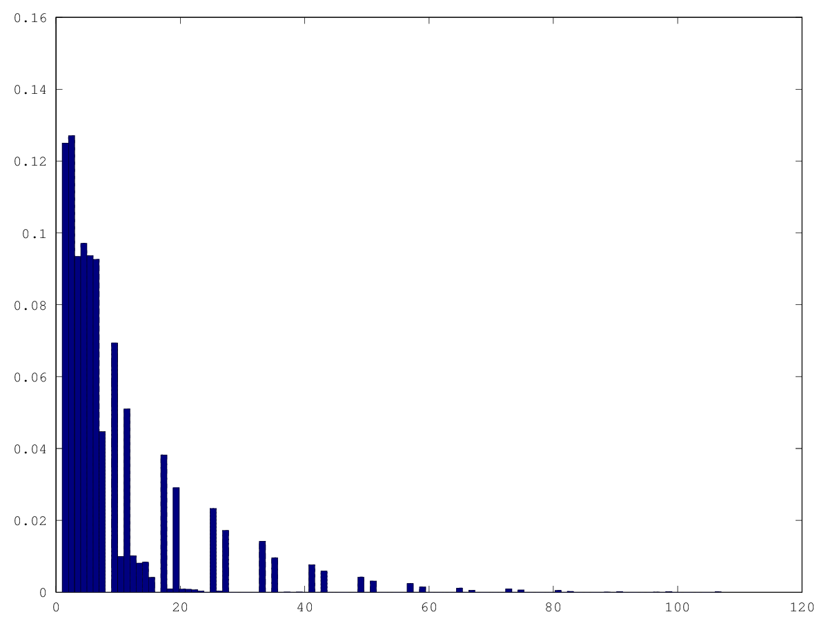
tries = dlmread("random_tries_pushsystematic_reduced.csv", ",", 0, 1);
hGramMatrix = [transpose(0:107), histc(tries, 0:107)];
csvwrite("systematic_reduced_histogram_counts.csv", hGramMatrix);
It appears as if any multiple of 8 (8, 16, 24, etc.) does not lead to an escape.
I will remove the 8th from the list of possible pushes.
diff -w -u1 box_pushsystematic_reduced.octave box_pushsystematic_reduced7.octave > diff5.patch
cat diff5.patch
--- box_pushsystematic_reduced.octave	2017-01-01 13:02:56.911733102 +0000
+++ box_pushsystematic_reduced7.octave	2017-01-01 13:17:12.967978056 +0000
@@ -3,4 +3,4 @@

-  while(index > 8)
-    index = index - 8;
+  while(index > 7)
+    index = index - 7;
   endwhile
@@ -13,4 +13,3 @@
 	       1, 0, 1, 0
-	       1, 0, 0, 1
-	       0, 0, 1, 1];
+	       1, 0, 0, 1];

@@ -62,3 +61,3 @@

-    csvwrite("random_tries_pushsystematic_reduced.csv", [startState, steps], "-append");
+    csvwrite("random_tries_pushsystematic_reduced7.csv", [startState, steps], "-append");
   endfor
octave box_pushsystematic_reduced7.octave
tries <- read.csv("random_tries_pushsystematic_reduced.csv", header=FALSE)
summary(tries$V2)
tries <- read.csv("random_tries_pushsystematic_reduced7.csv", header=FALSE)
summary(tries$V2)
 Min. 1st Qu.  Median    Mean 3rd Qu.    Max.
1.000   2.000   5.000   8.731  10.000 107.000
 Min. 1st Qu.  Median    Mean 3rd Qu.    Max.
1.000   2.000   5.000   8.091  10.000 101.000
graphics_toolkit("gnuplot")
tries = dlmread("random_tries_pushsystematic_reduced7.csv", ",", 0, 1)
hist(tries, 101, 1)
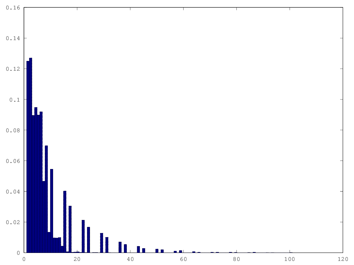
I notice that, after a point, only the button pushes 1 and 3 lead to escapes. What would happen if only those two were allowed?
diff -w -u1 box_pushsystematic_reduced7.octave box_pushsystematic_reduced2.octave > diff6.patch
cat diff6.patch
--- box_pushsystematic_reduced7.octave	2017-01-01 13:17:12.967978056 +0000
+++ box_pushsystematic_reduced2.octave	2017-01-01 15:16:44.851541506 +0000
@@ -3,13 +3,10 @@

-  while(index > 7)
-    index = index - 7;
-  endwhile
+  if (mod(index, 2) == 1)
+    index = 1;
+  else
+    index = 2;
+  endif

   allPushes = [1, 0, 0, 0
-	       0, 1, 0, 0
-	       0, 0, 1, 0
-	       0, 0, 0, 1
-	       1, 1, 0, 0
-	       1, 0, 1, 0
-	       1, 0, 0, 1];
+	       0, 0, 1, 0];

@@ -61,3 +58,3 @@

-    csvwrite("random_tries_pushsystematic_reduced7.csv", [startState, steps], "-append");
+    csvwrite("random_tries_pushsystematic_reduced2.csv", [startState, steps], "-append");
   endfor
octave box_pushsystematic_reduced2.octave
tries <- read.csv("random_tries.csv", header=FALSE)
summary(tries$V2)
tries <- read.csv("random_tries_pushsystematic_reduced7.csv", header=FALSE)
summary(tries$V2)
tries <- read.csv("random_tries_pushsystematic_reduced2.csv", header=FALSE)
summary(tries$V2)
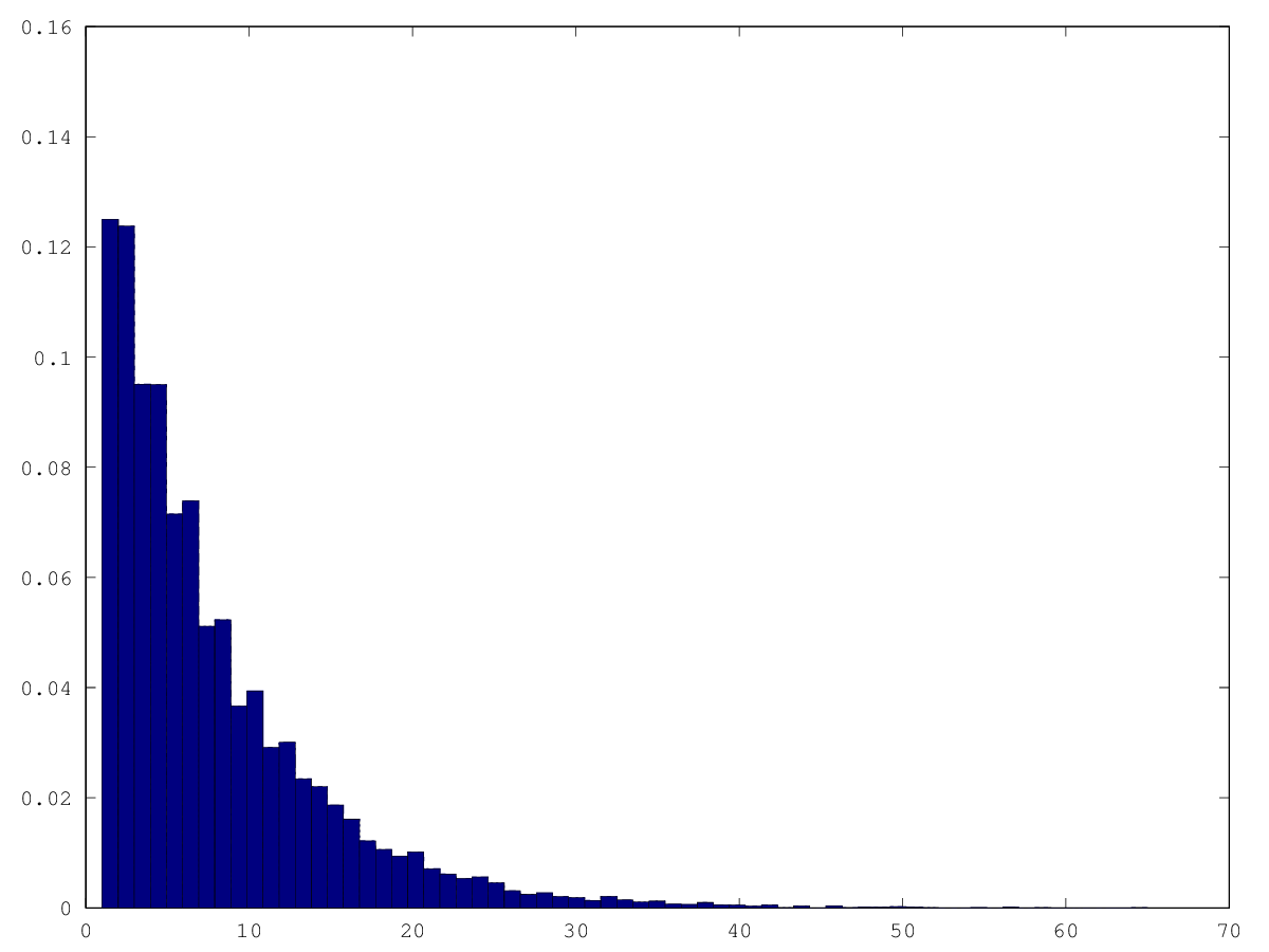
 Min. 1st Qu.  Median    Mean 3rd Qu.    Max.
1.000   3.000   5.000   7.285  10.000  74.000
 Min. 1st Qu.  Median    Mean 3rd Qu.    Max.
1.000   2.000   5.000   8.091  10.000 101.000
 Min. 1st Qu.  Median    Mean 3rd Qu.    Max.
1.000   3.000   5.000   7.442  10.000  65.000
Back to around "random" levels!
graphics_toolkit("gnuplot")
tries = dlmread("random_tries_pushsystematic_reduced2.csv", ",", 0, 1)
hist(tries, 65, 1)
![[FSF Associate Member]](/assets/fsf-12495.png)
![[FSFE Associate Member]](/assets/Button_Small_Fellow_No2744.png)